Fitting Attenuated RHESSI Spectra

Fitting attenuated RHESSI Spectra

This is looking at the M9 class flare observed by RHESSI from [Knuth+Glesener 2020](https://iopscience.iop.org/article/10.3847/1538-4357/abb779).

We perform spectroscopy on the interval where the thick attenuator is inserted.

Note

Systematic error is important to add to RHESSI data so that the minimizer has some wiggle room.

import matplotlib.pyplot as plt
import numpy as np
from parfive import Downloader

import astropy.time as atime

from sunkit_spex.extern import rhessi
from sunkit_spex.legacy.fitting import fitter

Download the example data

dl = Downloader()
base_url = "https://sky.dias.ie/public.php/dav/files/BHW6y6aXiGGosM6/rhessi/"
file_names = ["rhessi-2011-jul-stixbins-spec.fits", "rhessi-2011-jul-stixbins-srm.fits"]

for fname in file_names:
    dl.enqueue_file(base_url + fname, path="../../rhessi/")
files = dl.download()

Files Downloaded:   0%|          | 0/2 [00:00<?, ?file/s]

rhessi-2011-jul-stixbins-spec.fits:   0%|          | 0.00/395k [00:00<?, ?B/s]


rhessi-2011-jul-stixbins-srm.fits:   0%|          | 0.00/60.5k [00:00<?, ?B/s]

rhessi-2011-jul-stixbins-spec.fits:   0%|          | 1.02k/395k [00:00<01:02, 6.29kB/s]


rhessi-2011-jul-stixbins-srm.fits:   2%|▏         | 1.02k/60.5k [00:00<00:09, 6.37kB/s]

rhessi-2011-jul-stixbins-spec.fits:  11%|█         | 42.0k/395k [00:00<00:02, 135kB/s]


rhessi-2011-jul-stixbins-srm.fits:  69%|██████▉   | 42.0k/60.5k [00:00<00:00, 134kB/s]



Files Downloaded:  50%|█████     | 1/2 [00:00<00:00,  1.37file/s]

rhessi-2011-jul-stixbins-spec.fits:  54%|█████▍    | 214k/395k [00:00<00:00, 491kB/s]


Files Downloaded: 100%|██████████| 2/2 [00:00<00:00,  2.43file/s]
Files Downloaded: 100%|██████████| 2/2 [00:00<00:00,  2.17file/s]

Load in the spectrum and SRM, notice the warning about attenuator changes!

rl = rhessi.RhessiLoader(
    spectrum_fn="../../rhessi/rhessi-2011-jul-stixbins-spec.fits",
    srm_fn="../../rhessi/rhessi-2011-jul-stixbins-srm.fits",
)

/home/docs/checkouts/readthedocs.org/user_builds/sunkit-spex/conda/250/lib/python3.13/site-packages/sunkit_spex/extern/rhessi.py:196: UserWarning:
do not update event times to (2011-07-30T01:50:00.000, 2011-07-30T02:30:00.000): covers attenuator state change. Don't trust this fit!
  warnings.warn(

Notice there is no warning when the fit interval doesn’t cover an attenuator change!

rl.update_event_times(atime.Time("2011-07-30T02:08:20"), atime.Time("2011-07-30T02:10:20"))
end_background_time = "2011-07-30T01:56:00"
start_background_time = "2011-07-30T01:54:00"
rl.update_background_times(atime.Time(start_background_time), atime.Time(end_background_time))

Notice there is no warning when the fit interval doesn’t cover an attenuator change!

plt.figure()
rl.lightcurve(energy_ranges=[[4, 10], [10, 30], [30, 100]])

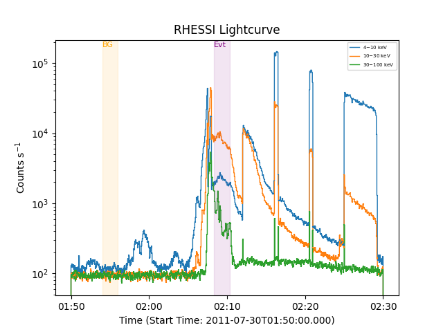
<Axes: title={'center': 'RHESSI Lightcurve'}, xlabel='Time (Start Time: 2011-07-30T01:50:00.000)', ylabel='Counts s$^{-1}$'>

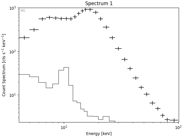
Add systematic error before passing to the fitter object

Uniform 10%

rl.systematic_error = 0.1

ss = fitter.Fitter(rl)
ss.energy_fitting_range = [5, 70]

plt.figure(layout="constrained")
axs, *_ = ss.plot()
_ = axs[0].set(xscale="log")

Define a custom model to and add to fitter.

def double_thick(electron_flux, low_index, break_energy, up_index, low_cutoff, up_cutoff, energies=None):
    from sunkit_spex.legacy.emission import bremsstrahlung_thick_target  # noqa: PLC0415

    mids = np.mean(energies, axis=1)
    flux = bremsstrahlung_thick_target(
        photon_energies=mids,
        p=low_index,
        eebrk=break_energy,
        q=up_index,
        eelow=low_cutoff,
        eehigh=up_cutoff,
    )

    # scale to good units
    return 1e35 * electron_flux * flux


ss.add_photon_model(double_thick, overwrite=True)

Prepare fit

ss.loglikelihood = "chi2"
ss.model = "f_vth + double_thick"

th_params = [
    "T1_spectrum1",
    "EM1_spectrum1",
]
nth_params = [
    "electron_flux1_spectrum1",
    "low_index1_spectrum1",
    "up_index1_spectrum1",
    "break_energy1_spectrum1",
    "low_cutoff1_spectrum1",
    "up_cutoff1_spectrum1",
]

ss.params["T1_spectrum1"] = ["free", 20, (5, 100)]
ss.params["EM1_spectrum1"] = ["free", 5000, (500, 100000)]

ss.params["electron_flux1_spectrum1"] = ["free", 10, (1, 50)]
ss.params["low_index1_spectrum1"] = ["free", 5, (1, 20)]
ss.params["up_index1_spectrum1"] = ["free", 5, (1, 20)]

ss.params["break_energy1_spectrum1"] = ["free", 40, (40, 100)]
ss.params["low_cutoff1_spectrum1"] = ["free", 20, (5, 39)]
ss.params["up_cutoff1_spectrum1"] = ["frozen", 500, (5, 1000)]

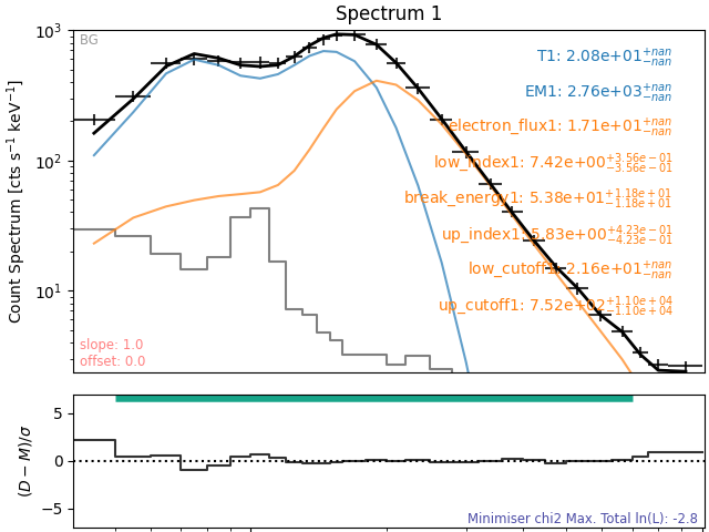
Fit the spectrum only varying the thermal params vary first

for p in th_params:
    ss.params[p] = "free"
for p in nth_params:
    ss.params[p] = "frozen"

_ = ss.fit()

Fit the spectrum only varying the non-thermal params vary first

for p in th_params:
    ss.params[p] = "frozen"
for p in nth_params:
    ss.params[p] = "free"

_ = ss.fit()

All params are free to vary

for p in th_params + nth_params:
    ss.params[p] = "free"

_ = ss.fit()

Plot

plt.figure(layout="constrained")
ss.plot()
plt.gca().set(xscale="log")

[None]

MCM (uncomment to run)

# ss.run_mcmc()