Note

Go to the end to download the full example code.

Fitting STIX Spectra#

Example of Fitting STIX Spectra#

This notebook provides a quick examples of STIX spectral fitting with sunkit-spex.

For a more explained demonstration of the general fitting process and other sunkit-spex capabilities see the NuSTAR and RHESSI fitting examples.

This is an example of how to perform a single STIX fit and a joint fit with STIX imaging and background detector spectra for when an attenuator is inserted. Therefore, in this example we use two spectral files from the same observation; one file contains spectrum from the imaging dectectors and the other file only uses the background detectors. You can obtain the files in a following way:

STIX science file (ID): 2410011252, STIX background file (ID): 2409216629

Preparation STIX spectrum (background subtracted) and SRM:

Routine stx_convert_pixel_data in the STIX GSW in IDL
- Input: science file and background file
- Output default: background subtracted spectrum of the 24 coarsest imaging detectors with all 8 big pixels (for each time step in the science file)
Imaging Detector spectrum for the 01.10.2024 flare: only top pixels should be used, additional keyword: pix_ind=[0,1,2,3]
BKG Detector spectrum for the 01.10.2024 flare: specific detector and pixel should be used, additional keywords: det_ind=[9], pix_ind=[2], /no_attenuation

Basic IDL code example:

stx_convert_pixel_data, fits_path_data = path_sci_file, fits_path_bk = path_bkg_file, $
    distance = distance, time_shift = time_shift, flare_location_stx = flare_location, $
    specfile = 'stx_spectrum_241001', srmfile = 'stx_srm_241001', plot=0 , $
    background_data = background_data, $ ospex_obj = ospex_obj

Imports

import matplotlib.pyplot as plt
from parfive import Downloader

import astropy.units as u
from astropy.time import Time

from sunkit_spex.extern.stix import STIXLoader
from sunkit_spex.legacy.fitting.fitter import Fitter, load

Download the example data

dl = Downloader()
base_url = "https://sky.dias.ie/public.php/dav/files/BHW6y6aXiGGosM6/stix/"
file_names = [
    "stx_spectrum_2410019944_IM.fits",
    "stx_srm_2410019944_IM.fits",
    "stx_spectrum_2410019944_BKG.fits",
    "stx_srm_2410019944_BKG.fits",
]

for fname in file_names:
    dl.enqueue_file(base_url + fname, path="../../stix/")
files = dl.download()

Files Downloaded:   0%|          | 0/4 [00:00<?, ?file/s]

stx_spectrum_2410019944_BKG.fits:   0%|          | 0.00/1.85M [00:00<?, ?B/s]

stx_spectrum_2410019944_IM.fits:   0%|          | 0.00/1.85M [00:00<?, ?B/s]

stx_srm_2410019944_IM.fits:   0%|          | 0.00/337k [00:00<?, ?B/s]

stx_srm_2410019944_BKG.fits:   0%|          | 0.00/179k [00:00<?, ?B/s]

stx_srm_2410019944_BKG.fits:   1%|          | 1.02k/179k [00:00<00:26, 6.76kB/s]

stx_srm_2410019944_IM.fits:   0%|          | 1.02k/337k [00:00<00:51, 6.49kB/s]

stx_spectrum_2410019944_BKG.fits:   0%|          | 1.02k/1.85M [00:00<04:49, 6.37kB/s]

stx_spectrum_2410019944_IM.fits:   0%|          | 1.02k/1.85M [00:00<04:50, 6.36kB/s]

stx_srm_2410019944_BKG.fits:  19%|█▉        | 33.8k/179k [00:00<00:00, 162kB/s]

stx_spectrum_2410019944_BKG.fits:   1%|          | 17.4k/1.85M [00:00<00:22, 80.4kB/s]

stx_srm_2410019944_BKG.fits:  32%|███▏      | 56.3k/179k [00:00<00:00, 188kB/s]

stx_srm_2410019944_IM.fits:  12%|█▏        | 42.0k/337k [00:00<00:02, 135kB/s]

stx_spectrum_2410019944_IM.fits:   2%|▏         | 42.0k/1.85M [00:00<00:13, 134kB/s]

stx_spectrum_2410019944_BKG.fits:   3%|▎         | 58.4k/1.85M [00:00<00:08, 212kB/s]

stx_srm_2410019944_BKG.fits:  65%|██████▍   | 116k/179k [00:00<00:00, 338kB/s]

stx_srm_2410019944_IM.fits:  37%|███▋      | 124k/337k [00:00<00:00, 350kB/s]

stx_spectrum_2410019944_IM.fits:   7%|▋         | 124k/1.85M [00:00<00:04, 350kB/s]

Files Downloaded:  25%|██▌       | 1/4 [00:00<00:02,  1.21file/s]

stx_spectrum_2410019944_BKG.fits:   6%|▋         | 116k/1.85M [00:00<00:05, 344kB/s]

stx_srm_2410019944_IM.fits:  88%|████████▊ | 296k/337k [00:00<00:00, 775kB/s]

stx_spectrum_2410019944_IM.fits:  16%|█▌        | 296k/1.85M [00:00<00:02, 774kB/s]

Files Downloaded:  50%|█████     | 2/4 [00:00<00:00,  2.51file/s]

stx_spectrum_2410019944_BKG.fits:  13%|█▎        | 239k/1.85M [00:00<00:02, 646kB/s]

stx_spectrum_2410019944_IM.fits:  30%|██▉       | 550k/1.85M [00:00<00:00, 1.32MB/s]

stx_spectrum_2410019944_BKG.fits:  28%|██▊       | 509k/1.85M [00:00<00:01, 1.32MB/s]

stx_spectrum_2410019944_IM.fits:  64%|██████▍   | 1.18M/1.85M [00:00<00:00, 2.83MB/s]

stx_spectrum_2410019944_BKG.fits:  56%|█████▋    | 1.04M/1.85M [00:00<00:00, 2.60MB/s]

Files Downloaded:  75%|███████▌  | 3/4 [00:01<00:00,  2.86file/s]

Files Downloaded: 100%|██████████| 4/4 [00:01<00:00,  3.27file/s]

Set up some plotting numbers

time_profile_size = (9, 6)
spec_plot_size = (10, 10)
joint_spec_plot_size = (25, 10)
tol = 1e-20
spec_font_size = 18
xlims, ylims = [3, 100], [1e-1, 1e6]

plt.rcParams["font.size"] = spec_font_size

The STIX loader is also able to automatically select an SRM based on the attenuator state during the time selected for sepctroscopy. In this example we select a time right before the attenuator is inserted. Load in the data…

stix_spec = STIXLoader(
    spectrum_file="../../stix/stx_spectrum_2410019944_IM.fits", srm_file="../../stix/stx_srm_2410019944_IM.fits"
)

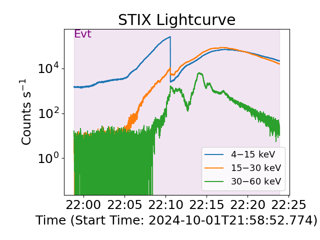
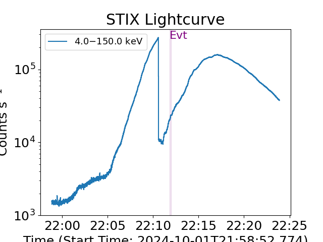
To see what we have, we can plot the time profile. The whole file time is taken as the event time as default (indicated by purple shaded region).

We do this by accessing the STIX spectral loader in the stix_spec.loaded_spec_data dictionary. Since the STIX spectrum is the only one loaded it is under the "spectrum1" entry.

Default energy range plotted is all energies but the user can define an energy rangem or ranges. Ranges are inclusive at the bounds and here we see the 4-15 keV, 15-30 keV, and 30-60 keV ranges.

plt.figure(layout="tight")

# the line that actually plots
stix_spec.lightcurve(energy_ranges=[[4, 15], [15, 30], [30, 60]])

plt.show()

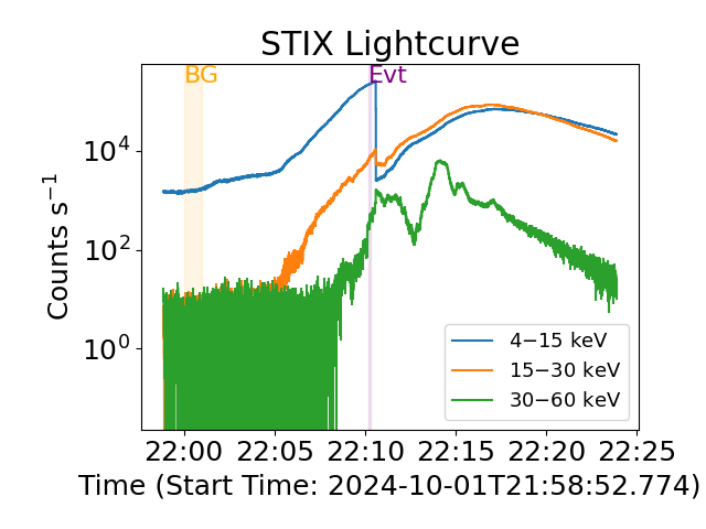
Since the default event data is assumed to be the full time, we might want to change this. In this particular case the background has been subtracted when the data was processes with IDL, therefore we don’t need to set a background time. To subtract background use the .update_background_times(start=.., end=..) method.

# Update event and bkg times
stix_spec.update_event_times(start=Time("2024-10-01T22:10:10"), end=Time("2024-10-01T22:10:18"))
stix_spec.update_background_times(start=Time("2024-10-01T22:00:00"), end=Time("2024-10-01T22:01:00"))
# Alternatively, you can select  the start and end event times in separate lines. e.g.
# stix_spec.start_event_time = "2024-10-01T22:10:10"
# stix_spec.end_event_time = "2024-10-01T22:10:18"

Plot again

plt.figure(layout="tight")
stix_spec.lightcurve(energy_ranges=[[4, 15], [15, 30], [30, 60]])
plt.show()

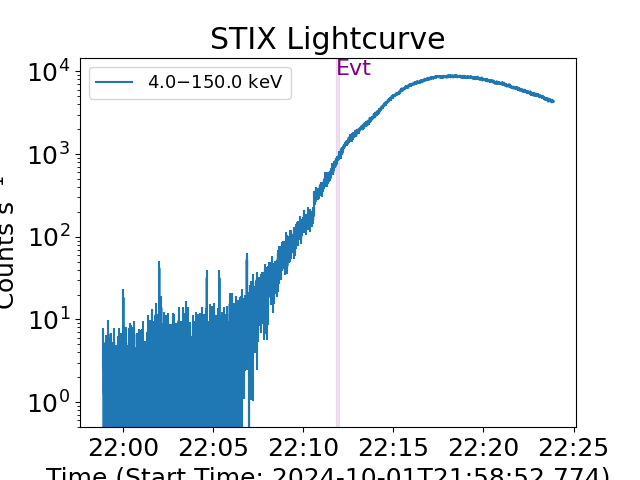
We can also see the X-ray evolution via a spectrogram.

# plot spectrogram
plt.figure(layout="tight")
stix_spec.spectrogram()
plt.show()

$STIX Spectrogram [Counts s$^{-1}$]$

Now let’s get going with a model and explicitly stating a fit statistic. For STIX analysis we choose chi2

fitter = Fitter(stix_spec)

fitter.model = "(f_vth + f_vth + thick_fn)"
fitter.loglikelihood = "chi2"

See what parameters we have to play with

fitter.show_params

Table masked=True length=8

Param	Status	Value	Bounds	Error
			(min, max)	(-, +)
str22	str10	float64	object	object
T1_spectrum1	free	1.00e+00	(0.0, None)	( 0.00e+00, 0.00e+00)
EM1_spectrum1	free	1.00e+00	(0.0, None)	( 0.00e+00, 0.00e+00)
T2_spectrum1	free	1.00e+00	(0.0, None)	( 0.00e+00, 0.00e+00)
EM2_spectrum1	free	1.00e+00	(0.0, None)	( 0.00e+00, 0.00e+00)
total_eflux1_spectrum1	free	1.00e+00	(0.0, None)	( 0.00e+00, 0.00e+00)
index1_spectrum1	free	1.00e+00	(0.0, None)	( 0.00e+00, 0.00e+00)
e_c1_spectrum1	free	1.00e+00	(0.0, None)	( 0.00e+00, 0.00e+00)
Fit Stat.	chi2 ln(L)	0.00e+00	--	--

Looking at the spectrum, define sensible numbers for starting values (maybe some trial and error here). For this spectrum, we will fit two thermals and non-thermal model over the whole energy range

fitter.energy_fitting_range = [4, 84]

# sort model parameters
fitter.params["T1_spectrum1"] = {"Value": 19, "Bounds": (13, 30), "Status": "free"}
fitter.params["EM1_spectrum1"] = {"Value": 470, "Bounds": (300, 800), "Status": "free"}
fitter.params["T2_spectrum1"] = {"Value": 40, "Bounds": (20, 60), "Status": "free"}
fitter.params["EM2_spectrum1"] = {"Value": 7, "Bounds": (3, 20), "Status": "free"}
fitter.params["total_eflux1_spectrum1"] = {"Value": 4, "Bounds": (1, 10), "Status": "free"}
fitter.params["index1_spectrum1"] = {"Value": 4, "Bounds": (2, 15), "Status": "free"}
fitter.params["e_c1_spectrum1"] = {"Value": 17, "Bounds": (10, 27), "Status": "free"}

Now perform the fit

# If you want to run the fit with MCMC you can use: fitter.run_mcmc(). See RHESSI or NuSTAR example notebook for how this can be done.

stix_spec_fit = fitter.fit(tol=tol)

The best-fit results

print(fitter.params)

                       Status  ...                                       Error
T1_spectrum1             free  ...    (0.5087872494315866, 0.5087872494315866)
EM1_spectrum1            free  ...      (49.00397378282912, 49.00397378282912)
T2_spectrum1             free  ...    (1.8675273835864603, 1.8675273835864603)
EM2_spectrum1            free  ...      (4.773480907118306, 4.773480907118306)
total_eflux1_spectrum1   free  ...    (2.7601062439047688, 2.7601062439047688)
index1_spectrum1         free  ...  (0.06362275664412424, 0.06362275664412424)
e_c1_spectrum1           free  ...    (0.9484577226030803, 0.9484577226030803)

[7 rows x 4 columns]

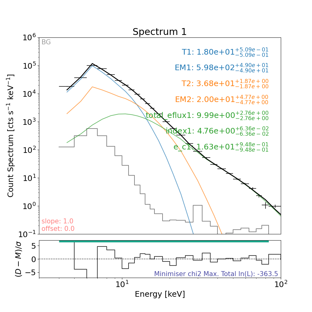
Let’s plot the result.

plt.figure(figsize=spec_plot_size)

# the line that actually plots
axes, res_axes = fitter.plot()

# make plot nicer
for a in axes:
    a.set_xlim(xlims)
    a.set_ylim(ylims)
    a.set_xscale("log")
plt.show()

Save out session#

save_filename = "../../stix/sunkitspexSTIXpectralFitting.pickle"
fitter.save(save_filename)

Loading session back in#

The session can be loaded back in using the following code as an example,

fitter_loaded = load(save_filename)

Let’s plot the result again

plt.figure(figsize=spec_plot_size)

# the line that actually plots
axes, res_axes = fitter_loaded.plot()

# make plot nicer
for a in axes:
    a.set_xlim(xlims)
    a.set_ylim(ylims)
    a.set_xscale("log")
plt.show()

Comparisons#

Model Parameter	Recent OSPEX Fit	This Work (MCMC, not shown)	This Work (normal fit)
T [MK]	19.61 $\pm$ 1.29	19.07 (-0.35, +0.26)	18.64 $\pm$ 0.22
EM [cm $^{-3}$ ]	471.90 $\pm$ 91.64 $\times$ $10^{46}$	484.15 (-17.55, +23.02) $\times$ $10^{46}$	554.37 $\pm$ 20.40 $\times$ $10^{46}$
Superhot T [MK]	42.36 $\pm$ 8.16	37.57 (-2.12, +1.61)	39.58 $\pm$ 0.96
Superhot EM [cm $^{-3}$ ]	7.70 $\pm$ 6.61 $\times$ $10^{46}$	13.70 (-2.46, +4.59) $\times$ $10^{46}$	13.55 $\pm$ 1.46 $\times$ $10^{46}$
e $^{-}$ Flux [e $^{-}$ s $^{-1}$ ]	4.41 $\pm$ 11.03 $\times$ $10^{35}$	5.35 (-0.76, +0.50) $\times$ $10^{35}$	9.99 $\pm$ 1.46 $\times$ $10^{35}$
Index	4.61 $\pm$ 0.17	4.71 (-0.05, +0.05)	4.74 $\pm$ 0.05
Low-E Cut-off [keV]	17.96 $\pm$ 12.74	17.88 (-0.57, +0.68)	16.09 $\pm$ 0.54

Joint fitting with background and imaging STIX detectors#

Loading the data into the fitter loader

spec_bg, srm_bg = "../../stix/stx_spectrum_2410019944_BKG.fits", "../../stix/stx_srm_2410019944_BKG.fits"
spec_im, srm_im = "../../stix/stx_spectrum_2410019944_IM.fits", "../../stix/stx_srm_2410019944_IM.fits"

spec_joint = Fitter(pha_file=[spec_bg, spec_im], srm_file=[srm_bg, srm_im])

Select time for integration

time_joint = ["2024-10-01T22:11:50", "2024-10-01T22:12:00"]
# Integrate the emission from the background detectors
spec_joint.data.loaded_spec_data["spectrum1"].update_event_times(start=time_joint[0], end=time_joint[1])
# Integrate the emission from the imaging detectors
spec_joint.data.loaded_spec_data["spectrum2"].update_event_times(start=time_joint[0], end=time_joint[1])

Plot the lightcurves

# For background detectors
plt.figure()
spec_joint.data.loaded_spec_data["spectrum1"].lightcurve()
plt.show()
# For imaging detectors
plt.figure()
spec_joint.data.loaded_spec_data["spectrum2"].lightcurve()
plt.show()

Define the energy range for fitting, the models to fit and the energy range

spec_joint.energy_fitting_range = {"spectrum1": [6, 25], "spectrum2": [11, 84]}

# Fitting two thermal models and a non-thermal model and a scaling factor
spec_joint.model = "C * (f_vth + f_vth + thick_fn)"

# Define the fit statistic to use
spec_joint.loglikelihood = "chi2"

# We added a scaling factor to account for systematic uncertainties
spec_joint.params["C_spectrum1"] = {"Value": 1, "Status": "fix"}
spec_joint.params["C_spectrum2"] = {"Value": 1, "Status": "free"}

Define the thermal models parameters

# Define the starting parameter values and boundaries
# The lower-T model mainly dominates in the background detectors spectrum so define them for spectrum 1
spec_joint.params["T1_spectrum1"] = {"Value": 20, "Bounds": (10, 30), "Status": "free"}
spec_joint.params["EM1_spectrum1"] = {"Value": 300, "Bounds": (200, 1000), "Status": "free"}

# Tie the parameters to spectrum 2
spec_joint.params["T1_spectrum2"] = spec_joint.params["T1_spectrum1"]
spec_joint.params["EM1_spectrum2"] = spec_joint.params["EM1_spectrum1"]

# The higher-T model dominates in the imaging detectors spectrum so define them for spectrum 2
spec_joint.params["T2_spectrum2"] = {"Value": 32, "Bounds": (30, 80), "Status": "free"}
spec_joint.params["EM2_spectrum2"] = {"Value": 500, "Bounds": (9, 800), "Status": "free"}

# Tie the parameters to spectrum 1
spec_joint.params["T2_spectrum1"] = spec_joint.params["T2_spectrum2"]
spec_joint.params["EM2_spectrum1"] = spec_joint.params["EM2_spectrum2"]

Define the non-thermal models parameters

# Fit the non-thermal model to imaging detectors
# electron flux param from thick_fn
spec_joint.params["total_eflux1_spectrum2"] = {"Value": 6, "Bounds": (0.9, 100), "Status": "free"}  # units 1e35 e^-/s
# electron index param from thick_fn
spec_joint.params["index1_spectrum2"] = {"Value": 5, "Bounds": (2, 10), "Status": "free"}
# electron low energy cut-off param from thick_fn
spec_joint.params["e_c1_spectrum2"] = {"Value": 20, "Bounds": (10, 30), "Status": "free"}  # units keV

# Tie non-thermal models fitted to spectrum 2 to spectrum 1
spec_joint.params["total_eflux1_spectrum1"] = spec_joint.params["total_eflux1_spectrum2"]
# electron index param from thick_fn
spec_joint.params["index1_spectrum1"] = spec_joint.params["index1_spectrum2"]
# electron low energy cut-off param from thick_fn
spec_joint.params["e_c1_spectrum1"] = spec_joint.params["e_c1_spectrum2"]

Add albedo

spec_joint.albedo_corr = True
spec_joint.albedo_angle = 76 * u.deg

Do the fit, this time we only use .fit() for this example to save compilation time. Since this is a complex fit, we recommend you run the full MCMC analysis to get reliable errors

spec_joint_fit = spec_joint.fit(tol=tol)

Files Downloaded:   0%|          | 0/1 [00:00<?, ?file/s]

green_compton_mu020.dat:   0%|          | 0.00/1.43M [00:00<?, ?B/s]

green_compton_mu020.dat:  95%|█████████▍| 1.36M/1.43M [00:00<00:00, 13.3MB/s]

Files Downloaded: 100%|██████████| 1/1 [00:00<00:00,  6.95file/s]
Files Downloaded: 100%|██████████| 1/1 [00:00<00:00,  6.91file/s]

Files Downloaded:   0%|          | 0/1 [00:00<?, ?file/s]

green_compton_mu025.dat:   0%|          | 0.00/1.43M [00:00<?, ?B/s]

green_compton_mu025.dat:  70%|██████▉   | 1.00M/1.43M [00:00<00:00, 9.74MB/s]

Files Downloaded: 100%|██████████| 1/1 [00:00<00:00,  6.07file/s]
Files Downloaded: 100%|██████████| 1/1 [00:00<00:00,  6.05file/s]

The best-fit results

print(spec_joint.params)

                                            Status  ...                                         Error
T1_spectrum1                                  free  ...                                    (nan, nan)
EM1_spectrum1                                 free  ...        (35.34136970897788, 35.34136970897788)
T2_spectrum1                      tie_T2_spectrum2  ...                                    (0.0, 0.0)
EM2_spectrum1                    tie_EM2_spectrum2  ...                                    (0.0, 0.0)
total_eflux1_spectrum1  tie_total_eflux1_spectrum2  ...                                    (0.0, 0.0)
index1_spectrum1              tie_index1_spectrum2  ...                                    (0.0, 0.0)
e_c1_spectrum1                  tie_e_c1_spectrum2  ...                                    (0.0, 0.0)
C_spectrum1                                 frozen  ...                                    (0.0, 0.0)
T1_spectrum2                      tie_T1_spectrum1  ...                                    (0.0, 0.0)
EM1_spectrum2                    tie_EM1_spectrum1  ...                                    (0.0, 0.0)
T2_spectrum2                                  free  ...    (0.40466913877776844, 0.40466913877776844)
EM2_spectrum2                                 free  ...                                    (nan, nan)
total_eflux1_spectrum2                        free  ...      (0.1950174722180021, 0.1950174722180021)
index1_spectrum2                              free  ...  (0.022763275018443174, 0.022763275018443174)
e_c1_spectrum2                                free  ...    (0.30467822706240777, 0.30467822706240777)
C_spectrum2                                   free  ...  (0.009583046758648609, 0.009583046758648609)

[16 rows x 4 columns]

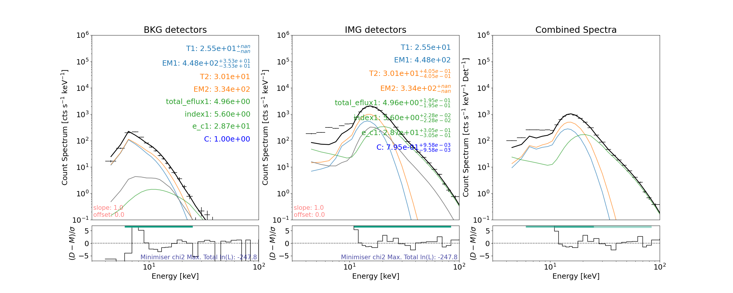
Let’s plot the result (the albedo is shown in grey)

plt.figure(figsize=joint_spec_plot_size)

# the line that actually plots
axes, res_axes = spec_joint.plot()

axes[0].set_title("BKG detectors")
axes[1].set_title("IMG detectors")

# make plot nicer
for a in axes:
    a.set_xlim(xlims)
    a.set_ylim(ylims)
    a.set_xscale("log")
plt.show()

BKG detectors, IMG detectors, Combined Spectra

Total running time of the script: (1 minutes 27.773 seconds)

Gallery generated by Sphinx-Gallery

Model Parameter	Recent OSPEX Fit	This Work (MCMC, not shown)	This Work (normal fit)
T [MK]	19.61 \(\pm\) 1.29	19.07 (-0.35, +0.26)	18.64 \(\pm\) 0.22
EM [cm \(^{-3}\) ]	471.90 \(\pm\) 91.64 \(\times\) \(10^{46}\)	484.15 (-17.55, +23.02) \(\times\) \(10^{46}\)	554.37 \(\pm\) 20.40 \(\times\) \(10^{46}\)
Superhot T [MK]	42.36 \(\pm\) 8.16	37.57 (-2.12, +1.61)	39.58 \(\pm\) 0.96
Superhot EM [cm \(^{-3}\) ]	7.70 \(\pm\) 6.61 \(\times\) \(10^{46}\)	13.70 (-2.46, +4.59) \(\times\) \(10^{46}\)	13.55 \(\pm\) 1.46 \(\times\) \(10^{46}\)
e \(^{-}\) Flux [e \(^{-}\) s \(^{-1}\) ]	4.41 \(\pm\) 11.03 \(\times\) \(10^{35}\)	5.35 (-0.76, +0.50) \(\times\) \(10^{35}\)	9.99 \(\pm\) 1.46 \(\times\) \(10^{35}\)
Index	4.61 \(\pm\) 0.17	4.71 (-0.05, +0.05)	4.74 \(\pm\) 0.05
Low-E Cut-off [keV]	17.96 \(\pm\) 12.74	17.88 (-0.57, +0.68)	16.09 \(\pm\) 0.54