Fitting Simulated Data

This is a file to show a very basic fitting of data where the model are generated in a different space (photon-space) which are converted using a square response matrix to the data-space (count-space).

Note

Caveats:

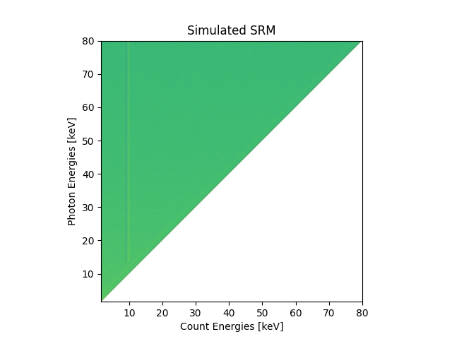
• The response is square so the count and photon energy axes are identical.

• No errors are included in the fitting statistic.

import matplotlib.pyplot as plt
import numpy as np
from matplotlib.colors import LogNorm

from astropy.modeling import fitting

from sunkit_spex.data.simulated_data import simulate_square_response_matrix
from sunkit_spex.fitting.objective_functions.optimising_functions import minimize_func
from sunkit_spex.fitting.optimizer_tools.minimizer_tools import scipy_minimize
from sunkit_spex.fitting.statistics.gaussian import chi_squared
from sunkit_spex.models.instrument_response import MatrixModel
from sunkit_spex.models.models import GaussianModel, StraightLineModel

Start by creating simulated data and instrument. This would all be provided by a given observation.

Can define the photon energies

start, inc = 1.6, 0.04
stop = 80 + inc / 2
ph_energies = np.arange(start, stop, inc)

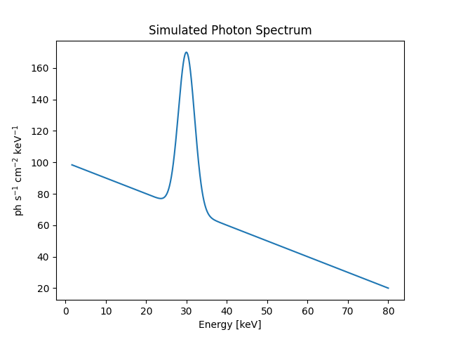
Let’s start making a simulated photon spectrum

sim_cont = {"edges": False, "slope": -1, "intercept": 100}
sim_line = {"edges": False, "amplitude": 100, "mean": 30, "stddev": 2}
# use a straight line model for a continuum, Gaussian for a line
ph_model = StraightLineModel(**sim_cont) + GaussianModel(**sim_line)

plt.figure()
plt.plot(ph_energies, ph_model(ph_energies))
plt.xlabel("Energy [keV]")
plt.ylabel("ph s$^{-1}$ cm$^{-2}$ keV$^{-1}$")
plt.title("Simulated Photon Spectrum")
plt.show()

Now want a response matrix

srm = simulate_square_response_matrix(ph_energies.size)
srm_model = MatrixModel(matrix=srm)

plt.figure()
plt.imshow(
    srm, origin="lower", extent=[ph_energies[0], ph_energies[-1], ph_energies[0], ph_energies[-1]], norm=LogNorm()
)
plt.ylabel("Photon Energies [keV]")
plt.xlabel("Count Energies [keV]")
plt.title("Simulated SRM")
plt.show()

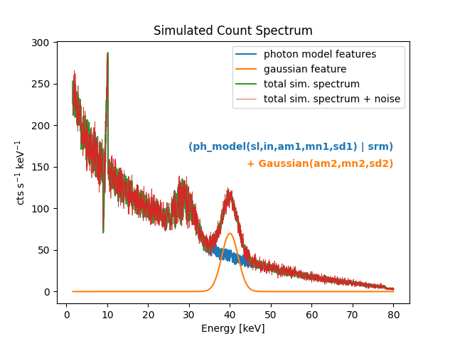
Start work on a count model

sim_gauss = {"edges": False, "amplitude": 70, "mean": 40, "stddev": 2}
# the brackets are very necessary
ct_model = (ph_model | srm_model) + GaussianModel(**sim_gauss)

Generate simulated count data to (almost) fit

sim_count_model = ct_model(ph_energies)

Add some noise

np_rand = np.random.default_rng(seed=10)
sim_count_model_wn = sim_count_model + (2 * np_rand.random(sim_count_model.size) - 1) * np.sqrt(sim_count_model)

Can plot all the different components in the simulated count spectrum

plt.figure()
plt.plot(ph_energies, (ph_model | srm_model)(ph_energies), label="photon model features")
plt.plot(ph_energies, GaussianModel(**sim_gauss)(ph_energies), label="gaussian feature")
plt.plot(ph_energies, sim_count_model, label="total sim. spectrum")
plt.plot(ph_energies, sim_count_model_wn, label="total sim. spectrum + noise", lw=0.5)
plt.xlabel("Energy [keV]")
plt.ylabel("cts s$^{-1}$ keV$^{-1}$")
plt.title("Simulated Count Spectrum")
plt.legend()

plt.text(80, 170, "(ph_model(sl,in,am1,mn1,sd1) | srm)", ha="right", c="tab:blue", weight="bold")
plt.text(80, 150, "+ Gaussian(am2,mn2,sd2)", ha="right", c="tab:orange", weight="bold")
plt.show()

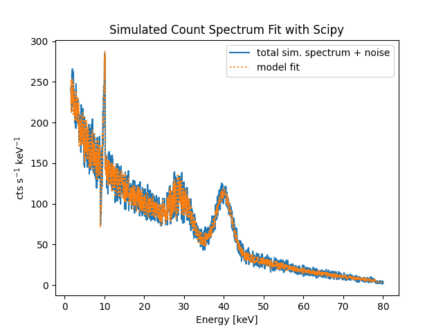
Now we have the simulated data, let’s start setting up to fit it

Get some initial guesses that are off from the simulated data above

guess_cont = {"edges": False, "slope": -0.5, "intercept": 80}
guess_line = {"edges": False, "amplitude": 150, "mean": 32, "stddev": 5}
guess_gauss = {"edges": False, "amplitude": 350, "mean": 39, "stddev": 0.5}

Define a new model since we have a rough idea of the mode we should use

ph_mod_4fit = StraightLineModel(**guess_cont) + GaussianModel(**guess_line)
count_model_4fit = (ph_mod_4fit | srm_model) + GaussianModel(**guess_gauss)

Let’s fit the simulated data and plot the result

opt_res = scipy_minimize(
    minimize_func, count_model_4fit.parameters, (sim_count_model_wn, ph_energies, count_model_4fit, chi_squared)
)

plt.figure()
plt.plot(ph_energies, sim_count_model_wn, label="total sim. spectrum + noise")
plt.plot(ph_energies, count_model_4fit.evaluate(ph_energies, *opt_res.x), ls=":", label="model fit")
plt.xlabel("Energy [keV]")
plt.ylabel("cts s$^{-1}$ keV$^{-1}$")
plt.title("Simulated Count Spectrum Fit with Scipy")
plt.legend()
plt.show()

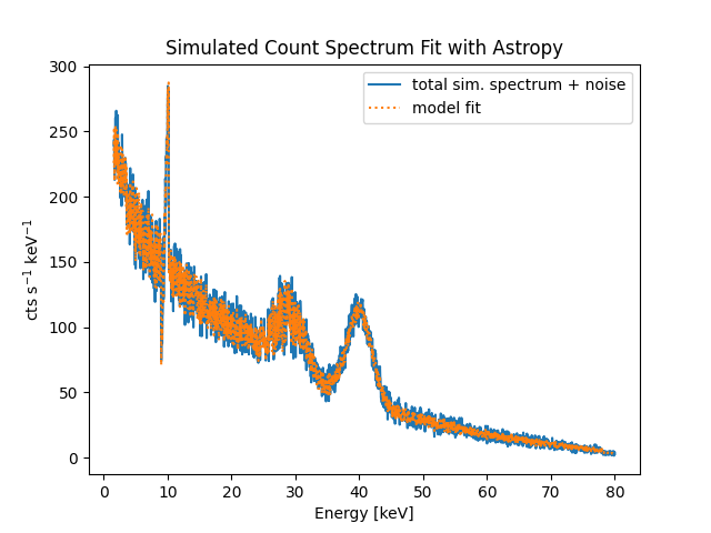
Now try and fit with Astropy native fitting infrastructure and plot the result

Try and ensure we start fresh with new model definitions

ph_mod_4astropyfit = StraightLineModel(**guess_cont) + GaussianModel(**guess_line)
count_model_4astropyfit = (ph_mod_4fit | srm_model) + GaussianModel(**guess_gauss)

astropy_fit = fitting.LevMarLSQFitter()

astropy_fitted_result = astropy_fit(count_model_4astropyfit, ph_energies, sim_count_model_wn)

plt.figure()
plt.plot(ph_energies, sim_count_model_wn, label="total sim. spectrum + noise")
plt.plot(ph_energies, astropy_fitted_result(ph_energies), ls=":", label="model fit")
plt.xlabel("Energy [keV]")
plt.ylabel("cts s$^{-1}$ keV$^{-1}$")
plt.title("Simulated Count Spectrum Fit with Astropy")
plt.legend()
plt.show()

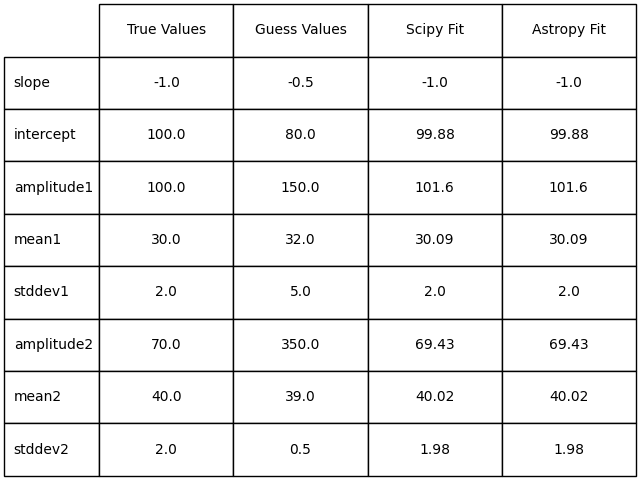
Display a table of the fitted results

plt.figure(layout="constrained")


row_labels = (
    tuple(sim_cont)[-2:] + tuple(f"{p}1" for p in tuple(sim_line)[-3:]) + tuple(f"{p}2" for p in tuple(sim_gauss)[-3:])
)
column_labels = ("True Values", "Guess Values", "Scipy Fit", "Astropy Fit")
true_vals = np.array(tuple(sim_cont.values())[-2:] + tuple(sim_line.values())[-3:] + tuple(sim_gauss.values())[-3:])
guess_vals = np.array(
    tuple(guess_cont.values())[-2:] + tuple(guess_line.values())[-3:] + tuple(guess_gauss.values())[-3:]
)
scipy_vals = opt_res.x
astropy_vals = astropy_fitted_result.parameters

print(np.shape(scipy_vals))
print(np.shape(astropy_vals))
print(np.shape(true_vals))
print(np.shape(guess_vals))

cell_vals = np.vstack((true_vals, guess_vals, scipy_vals, astropy_vals)).T
cell_text = np.round(np.vstack((true_vals, guess_vals, scipy_vals, astropy_vals)).T, 2).astype(str)

plt.axis("off")
plt.table(
    cellText=cell_text,
    cellColours=None,
    cellLoc="center",
    rowLabels=row_labels,
    rowColours=None,
    colLabels=column_labels,
    colColours=None,
    colLoc="center",
    bbox=[0, 0, 1, 1],
)

plt.show()

(8,)
(8,)
(8,)
(8,)