Note

Go to the end to download the full example code.

Fitting NuSTAR Spectra: Glesener et al. 2020 comparison#

A real example from [Glesener2020] of fitting two NuSTAR spectra simultaneously with gain correction.

import warnings

import matplotlib.pyplot as plt
import numpy as np
from numpy.exceptions import VisibleDeprecationWarning
from parfive import Downloader

from sunkit_spex.legacy.fitting.fitter import Fitter

warnings.filterwarnings("ignore", category=RuntimeWarning)
try:
    warnings.filterwarnings("ignore", category=VisibleDeprecationWarning)
except AttributeError:
    warnings.filterwarnings("ignore", category=np.exceptions.VisibleDeprecationWarning)

Set up some plotting numbers

spec_single_plot_size = (8, 10)
spec_plot_size = (25, 10)
spec_font_size = 18
default_font_size = 10
x_limits, y_limits = [1.6, 8.5], [1e-1, 1e3]

# Let’s fit a more realistic example

Try fitting the spectra presented in [Glesener et al. 2020](https://iopscience.iop.org/article/10.3847/2041-8213/ab7341). The spectrum presented shows clear evidence of non-thermal emission in an A5.7 microflare.

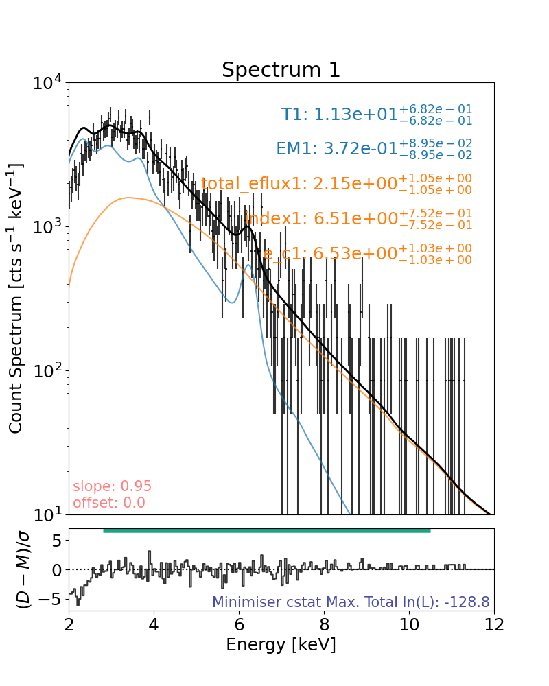
## Let’s recreate Figure 4 (left) where NuSTAR FPMB is fitted with a thermal+cold thick target model.

set up plotting info stuff

gles_xlims, gles_ylims = [2, 12], [1e1, 1e4]

Download data files

dl = Downloader()

base_url = "https://sky.dias.ie/public.php/dav/files/BHW6y6aXiGGosM6/nustar/Glesener2020/"
file_names = [
    "nu20312001001B06_cl_grade0_sr_grp.pha",
    "nu20312001001B06_cl_grade0_sr.arf",
    "nu20312001001B06_cl_grade0_sr.rmf",
    "nu20312001001A06_cl_grade0_sr_grp.pha",
    "nu20312001001A06_cl_grade0_sr.arf",
    "nu20312001001A06_cl_grade0_sr.rmf",
]

for fname in file_names:
    dl.enqueue_file(base_url + fname, path="../../nustar/Glesener2020/")
files = dl.download()

Files Downloaded:   0%|          | 0/6 [00:00<?, ?file/s]

nu20312001001B06_cl_grade0_sr.arf:   0%|          | 0.00/63.4k [00:00<?, ?B/s]

nu20312001001B06_cl_grade0_sr.rmf:   0%|          | 0.00/27.0M [00:00<?, ?B/s]

nu20312001001B06_cl_grade0_sr_grp.pha:   0%|          | 0.00/141k [00:00<?, ?B/s]

nu20312001001A06_cl_grade0_sr.arf:   0%|          | 0.00/63.4k [00:00<?, ?B/s]

nu20312001001A06_cl_grade0_sr_grp.pha:   0%|          | 0.00/141k [00:00<?, ?B/s]

nu20312001001B06_cl_grade0_sr.arf:   2%|▏         | 1.02k/63.4k [00:00<00:09, 6.64kB/s]

nu20312001001B06_cl_grade0_sr_grp.pha:   1%|          | 1.02k/141k [00:00<00:21, 6.54kB/s]

nu20312001001A06_cl_grade0_sr.arf:   2%|▏         | 1.02k/63.4k [00:00<00:09, 6.57kB/s]

nu20312001001B06_cl_grade0_sr.rmf:   0%|          | 1.02k/27.0M [00:00<1:13:07, 6.16kB/s]

nu20312001001A06_cl_grade0_sr_grp.pha:   1%|          | 1.02k/141k [00:00<00:23, 5.98kB/s]

nu20312001001B06_cl_grade0_sr_grp.pha:  18%|█▊        | 25.6k/141k [00:00<00:00, 121kB/s]

nu20312001001A06_cl_grade0_sr.arf:  53%|█████▎    | 33.8k/63.4k [00:00<00:00, 160kB/s]

nu20312001001B06_cl_grade0_sr.arf:  66%|██████▋   | 42.0k/63.4k [00:00<00:00, 137kB/s]

Files Downloaded:  17%|█▋        | 1/6 [00:00<00:03,  1.39file/s]

nu20312001001B06_cl_grade0_sr_grp.pha:  65%|██████▌   | 92.2k/141k [00:00<00:00, 341kB/s]

nu20312001001B06_cl_grade0_sr.rmf:   0%|          | 42.0k/27.0M [00:00<03:23, 132kB/s]

nu20312001001A06_cl_grade0_sr_grp.pha:  30%|██▉       | 42.0k/141k [00:00<00:00, 131kB/s]

nu20312001001B06_cl_grade0_sr_grp.pha:  94%|█████████▎| 132k/141k [00:00<00:00, 362kB/s]

Files Downloaded:  50%|█████     | 3/6 [00:00<00:00,  4.31file/s]

nu20312001001B06_cl_grade0_sr.rmf:   0%|          | 116k/27.0M [00:00<01:23, 321kB/s]

nu20312001001A06_cl_grade0_sr_grp.pha:  89%|████████▉ | 126k/141k [00:00<00:00, 350kB/s]

nu20312001001A06_cl_grade0_sr.rmf:   0%|          | 0.00/26.8M [00:00<?, ?B/s]

nu20312001001B06_cl_grade0_sr.rmf:   1%|          | 247k/27.0M [00:00<00:42, 626kB/s]

nu20312001001A06_cl_grade0_sr.rmf:   0%|          | 1.02k/26.8M [00:00<1:11:19, 6.26kB/s]

nu20312001001B06_cl_grade0_sr.rmf:   2%|▏         | 460k/27.0M [00:00<00:24, 1.09MB/s]

nu20312001001A06_cl_grade0_sr.rmf:   0%|          | 99.3k/26.8M [00:00<00:57, 461kB/s]

nu20312001001B06_cl_grade0_sr.rmf:   4%|▎         | 983k/27.0M [00:00<00:11, 2.35MB/s]

nu20312001001A06_cl_grade0_sr.rmf:   1%|          | 263k/26.8M [00:00<00:28, 929kB/s]

nu20312001001B06_cl_grade0_sr.rmf:   7%|▋         | 1.93M/27.0M [00:00<00:05, 4.51MB/s]

nu20312001001A06_cl_grade0_sr.rmf:   2%|▏         | 640k/26.8M [00:00<00:13, 1.96MB/s]

nu20312001001B06_cl_grade0_sr.rmf:  14%|█▍        | 3.89M/27.0M [00:00<00:02, 9.06MB/s]

nu20312001001A06_cl_grade0_sr.rmf:   5%|▌         | 1.40M/26.8M [00:00<00:06, 3.86MB/s]

nu20312001001B06_cl_grade0_sr.rmf:  28%|██▊       | 7.69M/27.0M [00:01<00:01, 17.3MB/s]

nu20312001001A06_cl_grade0_sr.rmf:  11%|█         | 2.90M/26.8M [00:00<00:03, 7.49MB/s]

nu20312001001B06_cl_grade0_sr.rmf:  41%|████      | 11.1M/27.0M [00:01<00:00, 20.8MB/s]

nu20312001001A06_cl_grade0_sr.rmf:  21%|██        | 5.50M/26.8M [00:00<00:01, 13.3MB/s]

nu20312001001B06_cl_grade0_sr.rmf:  55%|█████▍    | 14.8M/27.0M [00:01<00:00, 23.7MB/s]

nu20312001001A06_cl_grade0_sr.rmf:  33%|███▎      | 8.90M/26.8M [00:00<00:00, 19.6MB/s]

nu20312001001B06_cl_grade0_sr.rmf:  69%|██████▉   | 18.6M/27.0M [00:01<00:00, 25.4MB/s]

nu20312001001A06_cl_grade0_sr.rmf:  47%|████▋     | 12.6M/26.8M [00:01<00:00, 23.0MB/s]

nu20312001001B06_cl_grade0_sr.rmf:  83%|████████▎ | 22.3M/27.0M [00:01<00:00, 26.6MB/s]

nu20312001001A06_cl_grade0_sr.rmf:  61%|██████▏   | 16.4M/26.8M [00:01<00:00, 25.0MB/s]

nu20312001001B06_cl_grade0_sr.rmf:  97%|█████████▋| 26.1M/27.0M [00:01<00:00, 27.4MB/s]

Files Downloaded:  83%|████████▎ | 5/6 [00:02<00:00,  2.27file/s]

nu20312001001A06_cl_grade0_sr.rmf:  75%|███████▌  | 20.2M/26.8M [00:01<00:00, 26.3MB/s]

nu20312001001A06_cl_grade0_sr.rmf:  89%|████████▉ | 23.9M/26.8M [00:01<00:00, 27.3MB/s]

Files Downloaded: 100%|██████████| 6/6 [00:02<00:00,  2.66file/s]
Files Downloaded: 100%|██████████| 6/6 [00:02<00:00,  2.59file/s]

First, load in your data files, here we load in 2 spectra

_dir = "../../nustar/Glesener2020/"
# In the files here, the ARF and RMF file have different names to the PHA files so cannot use the PHA file name to help find the others so...
spec = Fitter(
    pha_file=_dir + "nu20312001001B06_cl_grade0_sr_grp.pha",
    arf_file=_dir + "nu20312001001B06_cl_grade0_sr.arf",
    rmf_file=_dir + "nu20312001001B06_cl_grade0_sr.rmf",
)

Define model, here we go for a single isothermal model + cold thick model

spec.model = "f_vth + thick_fn"

Define fitting range

spec.energy_fitting_range = [2.8, 10.5]

Sort temperature param from f_vth

spec.params["T1_spectrum1"] = {"Value": 10.3, "Bounds": (1.1, 15)}
# emission measure param from f_vth
spec.params["EM1_spectrum1"] = {"Value": 0.5, "Bounds": (1e-2, 1e1)}
# electron flux param from thick_fn
spec.params["total_eflux1_spectrum1"] = {"Value": 2.1, "Bounds": (1e-3, 10)}  # units 1e35 e^-/s
# electron index param from thick_fn
spec.params["index1_spectrum1"] = {"Value": 6.2, "Bounds": (3, 10)}
# electron low energy cut-off param from thick_fn
spec.params["e_c1_spectrum1"] = {"Value": 6.2, "Bounds": (1, 12)}  # units keV

This fit requires altering the gain parameters

Gain parameters can be tweaked in the same way model parameters can.

The difference is that gain parameters all have specific starting values (slope=1, offset=0) and are frozen by default.

# from Glesener et al. 2020 which had a gain correction fixed at 0.95
spec.rParams["gain_slope_spectrum1"] = {"Status": "fixed", "Value": 0.95}

print(spec.rParams)

print(spec.show_rParams)

                       Status  Value       Bounds       Error
gain_slope_spectrum1   frozen   0.95   (0.8, 1.2)  (0.0, 0.0)
gain_offset_spectrum1  frozen   0.00  (-0.1, 0.1)  (0.0, 0.0)
        Param         Status   Value       Bounds            Error
                                         (min, max)          (-, +)
--------------------- ------ ---------- ----------- ------------------------
 gain_slope_spectrum1 frozen      0.950  (0.8, 1.2) (      0.00,       0.00)
gain_offset_spectrum1 frozen      0.000 (-0.1, 0.1) (      0.00,       0.00)

Fit the model to the spectrum

spec.fit(tol=1e-8)

# Plot the result
plt.rcParams["font.size"] = spec_font_size
plt.figure(figsize=spec_single_plot_size)
axes, res_axes = spec.plot()
for a in axes:
    a.set_xlim(gles_xlims)
    a.set_ylim(gles_ylims)
plt.show()
plt.rcParams["font.size"] = default_font_size

Let’s recreate something similar to Figure 3(c)

Both NuSTAR FPMs are fitted with a thermal+cold thick target model simultaneously.

In the original Figure 3(c), a broken power law is used as the cold thick target does not exist ins XPSEC.

First, load in your data files, here we load in 2 spectra

_dir = "../../nustar/Glesener2020/"
spec = Fitter(
    pha_file=[_dir + "nu20312001001A06_cl_grade0_sr_grp.pha", _dir + "nu20312001001B06_cl_grade0_sr_grp.pha"],
    arf_file=[_dir + "nu20312001001A06_cl_grade0_sr.arf", _dir + "nu20312001001B06_cl_grade0_sr.arf"],
    rmf_file=[_dir + "nu20312001001A06_cl_grade0_sr.rmf", _dir + "nu20312001001B06_cl_grade0_sr.rmf"],
)

Define model, here we go for a single isothermal model + cold thick model

spec.model = "C*(f_vth + thick_fn)"

Define fitting range

spec.energy_fitting_range = [2.8, 10.5]

Sort temperature param from f_vth

spec.params["T1_spectrum1"] = {"Value": 10.3, "Bounds": (1.1, 15)}
# emission measure param from f_vth
spec.params["EM1_spectrum1"] = {"Value": 0.5, "Bounds": (1e-2, 1e1)}
# electron flux param from thick_fn
spec.params["total_eflux1_spectrum1"] = {"Value": 2.1, "Bounds": (1e-3, 10)}  # units 1e35 e^-/s
# electron index param from thick_fn
spec.params["index1_spectrum1"] = {"Value": 6.2, "Bounds": (3, 10)}
# electron low energy cut-off param from thick_fn
spec.params["e_c1_spectrum1"] = {"Value": 6.2, "Bounds": (1, 12)}  # units keV
# constant for systematic offset between FPMs, found to be about 1.1
spec.params["C_spectrum1"] = "frozen"
# constant for systematic offset between FPMs, found to be about 1.1
spec.params["C_spectrum2"] = {"Status": "fixed", "Value": 1.1}
# from Gles. 2020 which had a gain correction fixed at 0.95
spec.rParams["gain_slope_spectrum1"] = {"Status": "fixed", "Value": 0.95}
spec.rParams["gain_slope_spectrum2"] = spec.rParams["gain_slope_spectrum1"]

Fit the model to the spectrum

spec.fit(tol=1e-8)

# Plot the result
plt.rcParams["font.size"] = spec_font_size
plt.figure(figsize=spec_plot_size)
axes, res_axes = spec.plot()
for a in axes:
    a.set_xlim(gles_xlims)
    a.set_ylim(gles_ylims)
plt.show()
plt.rcParams["font.size"] = default_font_size

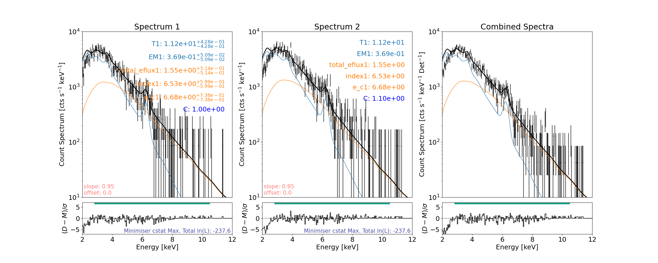
Spectrum 1, Spectrum 2, Combined Spectra

For the thermal and cold thick target total model we compare

Model Parameter	OSPEX (Glesener et al. 2020) [*]	This Work (just FPMB)	This Work (FPMA&B)
Temperature [MK]	10.3$\pm$0.7	11.3$\pm$0.7	11.2$\pm$0.4
Emission Measure [cm^-3]	5.0 $\pm$ 1.3$\times$10 ⁴⁵	3.7 $\pm$ 0.9$\times$10 ⁴⁵	3.7 $\pm$ 0.5$\times$10 ⁴⁵
Electron Flux [e$^{-}$ s$^{-1}$]	2.1$\pm$1.1$\times$10 ³⁵	2.2$\pm$1.1$\times$10 ³⁵	1.6$\pm$0.5$\times$10 ³⁵
Index	6.2$\pm$0.6	6.5$\pm$0.8	6.5$\pm$0.6
Low Energy Cut-off [keV]	6.2$\pm$0.9	6.5$\pm$1.0	6.7$\pm$0.7

[Glesener2020]

https://iopscience.iop.org/article/10.3847/2041-8213/ab7341

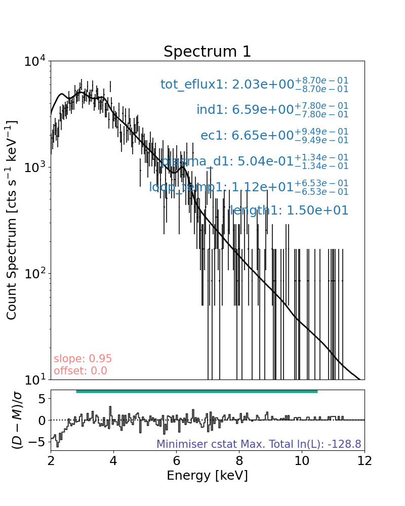
Now let’s recreate Figure 4 (right)

NuSTAR FPMB is fitted with a warm thick target model.

The warm thick target model helps to constrain the non-thermal emission with observed values (e.g., loop length, etc) and ties it to the thermal emission parameters.

First, load in your data files, here we load in 1 spectrum

_dir = "../../nustar/Glesener2020/"
spec = Fitter(
    pha_file=_dir + "nu20312001001B06_cl_grade0_sr_grp.pha",
    arf_file=_dir + "nu20312001001B06_cl_grade0_sr.arf",
    rmf_file=_dir + "nu20312001001B06_cl_grade0_sr.rmf",
)

define model, here we go for a single isothermal model + cold thick model

spec.model = "thick_warm"

define fitting range

spec.energy_fitting_range = [2.8, 10.5]

# electron flux param
spec.params["tot_eflux1_spectrum1"] = {"Value": 2, "Bounds": (1e-2, 10)}
# electron index param
spec.params["ind1_spectrum1"] = {"Value": 6, "Bounds": (3, 10)}
# electron low energy cut-off param
spec.params["ec1_spectrum1"] = {"Value": 7, "Bounds": (3, 12)}
# loop plasma temperature param
spec.params["loop_temp1_spectrum1"] = {"Value": 10, "Bounds": (5, 15)}
# plasma number density param
spec.params["plasma_d1_spectrum1"] = {"Value": 1, "Bounds": (1e-2, 1e1)}  # units 1e10 cm^-3
# loop length param
spec.params["length1_spectrum1"] = {"Status": "fixed", "Value": 15}  # units Mm
# from Gles. 2020 which had a gain correction fixed at 0.95
spec.rParams["gain_slope_spectrum1"] = {"Status": "fixed", "Value": 0.95}

fit the model to the spectrum

spec.fit(tol=1e-10)

# plot the result
plt.rcParams["font.size"] = spec_font_size
plt.figure(figsize=spec_single_plot_size)
axes, res_axes = spec.plot()
for a in axes:
    a.set_xlim(gles_xlims)
    a.set_ylim(gles_ylims)
plt.show()
plt.rcParams["font.size"] = default_font_size

Minimum length>length

Fitting the warm thick target model to both FPMs simultaneously

First, load in your data files, here we load in 2 spectra

_dir = "../../nustar/Glesener2020/"
spec = Fitter(
    pha_file=[_dir + "nu20312001001A06_cl_grade0_sr_grp.pha", _dir + "nu20312001001B06_cl_grade0_sr_grp.pha"],
    arf_file=[_dir + "nu20312001001A06_cl_grade0_sr.arf", _dir + "nu20312001001B06_cl_grade0_sr.arf"],
    rmf_file=[_dir + "nu20312001001A06_cl_grade0_sr.rmf", _dir + "nu20312001001B06_cl_grade0_sr.rmf"],
)

Define model, here we go for a single isothermal model + cold thick model

spec.model = "C*thick_warm"

Define fitting range

spec.energy_fitting_range = [2.8, 10.5]

# electron flux param
spec.params["tot_eflux1_spectrum1"] = {"Value": 2, "Bounds": (1e-3, 10)}
# electron index param
spec.params["ind1_spectrum1"] = {"Value": 6, "Bounds": (3, 10)}
# electron low energy cut-off param
spec.params["ec1_spectrum1"] = {"Value": 7, "Bounds": (1, 12)}
# loop plasma temperature param
spec.params["loop_temp1_spectrum1"] = {"Value": 10, "Bounds": (1.1, 15)}
# plasma number density param
spec.params["plasma_d1_spectrum1"] = {"Value": 1, "Bounds": (1e-2, 1e1)}
# loop length param
spec.params["length1_spectrum1"] = {"Status": "fixed", "Value": 15}
# constant for systematic offset between FPMs, found to be about 1.1
spec.params["C_spectrum1"] = "frozen"
spec.params["C_spectrum2"] = {"Status": "fixed", "Value": 1.1}
# from Gles. 2020 which had a gain correction fixed at 0.95
spec.rParams["gain_slope_spectrum1"] = {"Status": "fixed", "Value": 0.95}
spec.rParams["gain_slope_spectrum2"] = spec.rParams["gain_slope_spectrum1"]

Fit the model to the spectrum

spec.fit(tol=1e-5)

# Plot the result
plt.rcParams["font.size"] = spec_font_size
plt.figure(figsize=spec_plot_size)
axes, res_axes = spec.plot()
for a in axes:
    a.set_xlim(gles_xlims)
    a.set_ylim(gles_ylims)
plt.show()
plt.rcParams["font.size"] = default_font_size

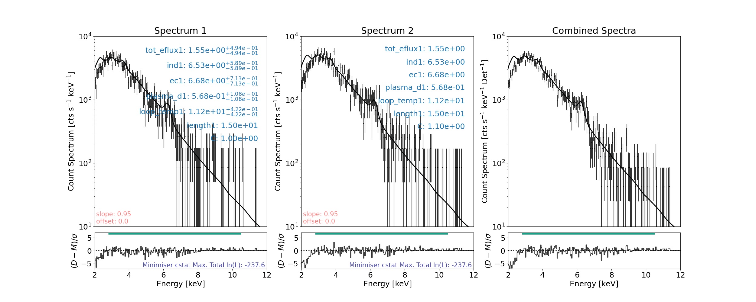
For warm thick target total model we compare

Model Parameter	OSPEX (Glesener et al. 2020)	This Work (just FPMB)	This Work (FPMA&B)
Temperature [MK]	10.2$\pm$0.7	11.2$\pm$0.6	11.2$\pm$0.4
Plasma Density [cm^-3]	6.0 $\pm$ 2.0$\times$10 ⁹	5.0 $\pm$ 1.3$\times$10 ⁹	5.7 $\pm$ 1.1$\times$10 ⁹
Electron Flux [e$^{-}$ s$^{-1}$]	1.8$\pm$0.8$\times$10 ³⁵	2.0$\pm$0.8$\times$10 ³⁵	1.6$\pm$0.5$\times$10 ³⁵
Index	6.3$\pm$0.7	6.6$\pm$0.8	6.5$\pm$0.6
Low Energy Cut-off [keV]	6.5$\pm$0.9	6.7$\pm$0.9	6.7$\pm$0.7

All parameter values appear to be within error margins (or extremely close). This is more impressive when the errors calculated in this work for the minimised values assumes the parameter’s have a Gaussian and independent posterior distribution (which is clearly not the case) and so these errors are likely to be larger; to be investigated with an MCMC.

The simultaneous fit of FPMA&B with the cold thick target model and the warm thick model is not able to be performed in OSPEX.

Total running time of the script: (2 minutes 16.829 seconds)

Gallery generated by Sphinx-Gallery

Model Parameter	OSPEX (Glesener et al. 2020) [*]	This Work (just FPMB)	This Work (FPMA&B)
Temperature [MK]	10.3\(\pm\)0.7	11.3\(\pm\)0.7	11.2\(\pm\)0.4
Emission Measure [cm^-3]	5.0 \(\pm\) 1.3\(\times\)10 ⁴⁵	3.7 \(\pm\) 0.9\(\times\)10 ⁴⁵	3.7 \(\pm\) 0.5\(\times\)10 ⁴⁵
Electron Flux [e$^{-}$ s$^{-1}$]	2.1\(\pm\)1.1\(\times\)10 ³⁵	2.2\(\pm\)1.1\(\times\)10 ³⁵	1.6\(\pm\)0.5\(\times\)10 ³⁵
Index	6.2\(\pm\)0.6	6.5\(\pm\)0.8	6.5\(\pm\)0.6
Low Energy Cut-off [keV]	6.2\(\pm\)0.9	6.5\(\pm\)1.0	6.7\(\pm\)0.7

Model Parameter	OSPEX (Glesener et al. 2020)	This Work (just FPMB)	This Work (FPMA&B)
Temperature [MK]	10.2\(\pm\)0.7	11.2\(\pm\)0.6	11.2\(\pm\)0.4
Plasma Density [cm^-3]	6.0 \(\pm\) 2.0\(\times\)10 ⁹	5.0 \(\pm\) 1.3\(\times\)10 ⁹	5.7 \(\pm\) 1.1\(\times\)10 ⁹
Electron Flux [e$^{-}$ s$^{-1}$]	1.8\(\pm\)0.8\(\times\)10 ³⁵	2.0\(\pm\)0.8\(\times\)10 ³⁵	1.6\(\pm\)0.5\(\times\)10 ³⁵
Index	6.3\(\pm\)0.7	6.6\(\pm\)0.8	6.5\(\pm\)0.6
Low Energy Cut-off [keV]	6.5\(\pm\)0.9	6.7\(\pm\)0.9	6.7\(\pm\)0.7